Lagrangian coherent structures for flows in 2-D/3-D Euclidean spaces
The MATLAB code to compute FTLE for flows defined on Euclidean spaces is available at this link. The following tutorial provides instructions on how to use the code. We use finite-differencing to approximate the deformation gradient and compute FTLE. The numerical method is described in [1].
Pre-requisites
The code was built on MATLAB R2025b in a Windows 10 system. We have tested these codes on a Mac OSX 15 and Ubuntu 20 operating systems. The most straightforwrd Installation method, is using Git, as all the code is hosted on GitHub. We assume that Git is installed and set up on the system. If not, we refer you to this link.
Installation
To install the code, navigate to the path where you would want to install it on the terminal and clone the GitHub repository using the code
git clone https://github.com/SreejithSanthosh/flow_coherent_structure.git
This will generate a directory called flow_coherent_structure, which contains all the code. To check if all the necessary components navigate to the ftle_from_euclidean_grid folder and make it your root directory in MATLAB and run example_euclideangrid2d.m on MATLAB. This runs the deformation analysis, presenting the results below for the double-gyre velocity field.
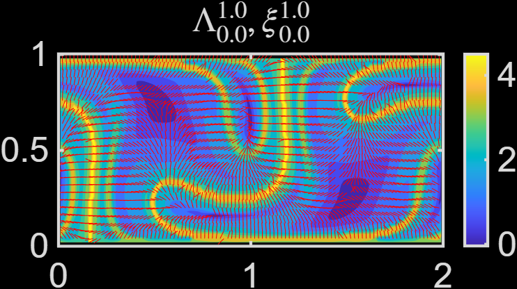
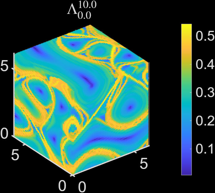
\(\Lambda\) is the FTLE field, \(\xi\) is the axis of maximum deformation. Similarly run example_euclideangrid3d.m on MATLAB to check if the code works for 3D flows. This runs the deformation analysis, presenting the results below for the ABC flow.
Further development of this code is currently ongoing to improve the robustness of the method and increase its speed. To get those updates, use the command
git pull
Performing deformation analysis for your data
The two example codes for 2D and 3D flows which are example_euclidean2D.m and example_euclidean3D.m are written for a specific flow field. To use this analysis for your flow field, you need to advect a grid from the initial configuration at time \(t_0\) to \(t_f\). For a 2D flow, the two coordinates of the intial grids x0, y0 are advected onto xf,yf. The function compute_deform_euclidean2d.m computes the singular values and its associated axis from x0,y0,xf,yf. From the results of this function, the FTLE can be visualized using the code described in %% Visualize the result in example_euclidean2D.m. Similarly for a 3D flow the intial grid defined by x0,y0,z0 is advected onto xf,yf,zf. The intial and final grids are passed through the function compute_deform_euclidean3d.m the result from which the FTLE can be visualized.
References
[1] : Haller, G., 2015. Lagrangian coherent structures. Annual review of fluid mechanics, 47(1)