Lagrangian Coherent Structures from Sparse and Noisy Trajectories in 2D/3D Euclidean Spaces

This tutorial explains how to use the MATLAB code for computing finite-time Lyapunov exponent (FTLE) fields from sparse and noisy trajectory data in 2D and 3D Euclidean spaces. The MATLAB code is available in the GitHub repository: flow_coherent_structure. The method is designed for cases where the full velocity field is not available, but particle or material trajectories are known at an initial and final time. The numerical method follows the approach described in [1].

Prerequisites

The code was developed using MATLAB R2025b on a Windows 10 system. It has also been tested on:

• macOS 15
• Ubuntu 20

The recommended installation method is through Git, since the code is hosted on GitHub. This tutorial assumes that Git is already installed and configured on your system. If Git is not installed, follow the installation instructions here: Installing Git

Installation

Navigate to the directory where you want to install the code, then clone the GitHub repository:

git clone https://github.com/SreejithSanthosh/flow_coherent_structure.git

This command creates a directory called:

flow_coherent_structure

which contains the MATLAB scripts, functions, and example files. To test the sparse-trajectory FTLE code, navigate to the folder:

ftle_from_sparse_trajec

and set it as the root directory in MATLAB.

Example: Sparse Trajectories from a 2D Double-Gyre Flow

To test the code, run the following MATLAB script:

example_sparsetrajec2d.m

This script performs the deformation analysis using sparse trajectory data generated from the 2D double-gyre velocity field. The output is shown below.

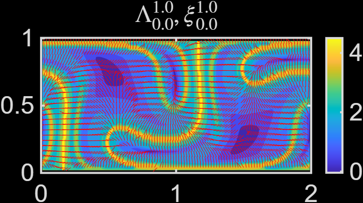
Here:

• $\Lambda$ is the FTLE field.
• $\xi$ is the axis of maximum deformation.

Updating the Code

The code is under active development. To update your local copy with the latest changes, navigate to the repository directory and run:

git pull

Performing Deformation Analysis on Your Own Trajectory Data

The example script example_sparsetrajec2d.m is written for a specific test flow. To apply the analysis to your own data, you need the initial and final positions of a set of trajectories. The Lagrangian analysis is performed over the time interval $t_0$ to $t_f$. For each trajectory, the code requires its initial position at time $t_0$ and its final position at time $t_f$. The deformation metrics are computed using:

compute_deform_sparsetrajec.m

This function estimates the singular values of the deformation gradient and the corresponding deformation axes from the sparse trajectory data.

2D/3D Trajectory Data Format

The example script example_sparsetrajec2d.m is written for a specific flow field. To apply this analysis to your own data, you need the initial and final positions of the trajectories over the time interval \(t_0 \rightarrow t_f\).

For a 2D flow, the initial trajectory coordinates x0, y0 at time \(t_0\) are advected to the final coordinates xf, yf at time \(t_f\). These coordinates are formatted as r0 and rf, which are then passed to compute_deform_sparsetrajec.m. This function computes the singular values and their associated directions from the initial and final trajectory positions. The resulting FTLE field can then be visualized using the code provided in the %% Visualize the result section of example_sparsetrajec2d.m.

The function compute_deform_sparsetrajec.m can also compute deformation metrics for 3D trajectories. In this case, r0 and rf should be formatted as double arrays of size Nq x 3, where Nq is the number of trajectories and the three columns correspond to the three spatial coordinates of each trajectory.

Summary of Workflow

The general workflow for computing FTLE fields from sparse and noisy trajectories is:

1. Collect or generate trajectory data.
2. Store the initial trajectory positions at time $t_0$ in r0.
3. Store the corresponding final trajectory positions at time $t_f$ in rf.
4. Pass r0 and rf to compute_deform_sparsetrajec.m.
5. Compute the singular values and deformation axes.
6. Visualize the FTLE field and the axis of maximum deformation.

This method is especially useful when the full velocity field is unavailable, but trajectory data are available from experiments, simulations, or particle-tracking measurements.

---

References

[1] Mowlavi, S., Serra, M., Maiorino, E., & Mahadevan, L. (2022). Detecting Lagrangian coherent structures from sparse and noisy trajectory data. Journal of Fluid Mechanics, 948, A4.